오차 역전파법 -1

수치미분 vs 연쇄법칙 + 미분공식

수치미분

수치미분

연쇄법칙 + 미분공식

연쇄법칙 + 미분공식

 

 

예제

합성

 

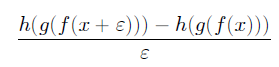
수치미분을 이용한 식:

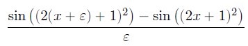
연쇄 법칙 + 미분공식을 이용한 식:

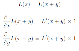
오차 역전파법에서는 연쇄 법칙 + 미분 공식을 이용한다.

여기서 '역전파'라는 이름이 붙은 이유는 미분을 하는 순서가 합성함수를 취하는 순서의 역이기 때문!

(합성은 f -> g -> h 순서, 미분은 h -> g -> f 순서로 진행)

---

그래프

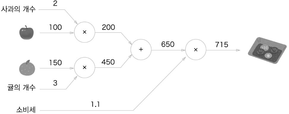
graph

계산 그래프 : 순전파

사과 개당 가격 : 100, 사과 개수: 2 

귤 개당 가격: 150, 귤 개수: 3 소비세 : 10%

지불 금액 : (100  x 2 + 150 x 3) x 1.1 = 715

계산 그래프 : 순전파

 

계산 그래프 : 역전파

1로 출발해서 오른쪽에서 왼쪽으로 흘러간다.

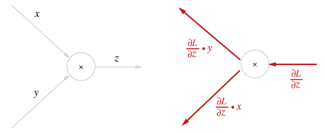
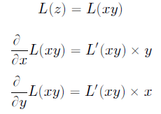
곱셈노드 : 반대편 값을 엇갈려서 곱해서 흘려보낸다.

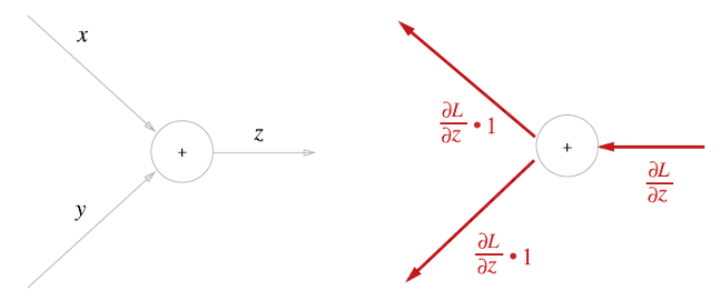
덧셈노드 : 그냥 흘려보낸다.

계산 그래프 : 역전파

 

 

역전파와 미분

사과 개당 가격 : x, 사과 개수 : m, 소비세 : t

귤 개당 가격: y, 귤 개수 : n, 소비세 : t

지불금액 : f(x,m,y,n,t) = (xm + yn)t

 

 

 

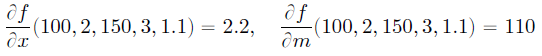
편미분의 결과와 그래프에 마지막에 나오는 값이 일치한다.

역전파의 결과는 각각의 변수를 기준으로 편미분한 결과라는 것을 알 수 있다.

 

덧셈 노드의 역전파

곱셈 노드의 역전파

---

파이썬 코드로 구현

위에서 살펴본 그래프 기반 역전파를 코드로 구현해보자.

먼저 곱셈노드의 역전파이다.

class MulLayer:
    def __init__(self):
        self.x = None
        self.y = None

    def forward(self, x, y):
        self.x = x
        self.y = y
        out = x * y

        return out

    def backward(self, dout):
        dx = dout * self.y
        dy = dout * self.x

        return dx, dy

forward(순전파) 메서드는 입력값 x, y를 곱하여 x * y를 반환해준다.

backward(역전파) 메서드는 x로 편미분한 값 dx, y로 편미분한 값 dy를 구하여 반환해준다.

 

덧셈 노드의 역전파

class AddLayer:
    def __init(self):
        pass

    def forward(self, x, y):
        out = x + y

        return out

    def backward(self, dout):
        dx = dout * 1
        dy = dout * 1

        return dx, dy

forward(순전파) 메서드는 입력값 x, y를 더하여 x + y를 반환해준다.

backward(역전파) 메서드는 x로 편미분한 값 dx, y로 편미분한 값 dy를 구하여 반환해준다.

 

위의 MulLayer, AddLayer를 이용하여 아래의 그래프를 코드로 구현해보자.

from layer_naive import *

apple_num = 2
orange_num = 3
apple = 100
orange = 150
tax = 1.1

mul_apple_layer = MulLayer()
mul_orange_layer = MulLayer()
add_apple_orange_layer = AddLayer()
mul_tax_layer = MulLayer()

# forward
apple_price = mul_apple_layer.forward(apple_num, apple)
orange_price = mul_orange_layer.forward(orange_num, orange)
total_price = add_apple_orange_layer.forward(apple_price, orange_price)
price = mul_tax_layer.forward(total_price, tax)

# backward
dprice = 1
dtotal_price, dtax = mul_tax_layer.backward(dprice)
dapple_price, dorange_price = add_apple_orange_layer.backward(dtotal_price)
dapple, dapple_num = mul_apple_layer.backward(dapple_price)
dorange, dorange_num = mul_apple_layer.backward(dorange_price)

print("price:", int(price))
print("dApple:", dapple)
print("dApple_num:", int(dapple_num))
print("dApple:", dorange)
print("dApple_num:", int(dorange_num))
print("dTax:", dtax)

 

 

 

 

이미지 출처 : https://drive.google.com/file/d/1UwEE_6f71RLA8DB5HGbflsXzxCWdqplD/view